The NPV formula in Excel is counterintuitive at first. When I first used it, I made a simple mistake by selecting all the cash flow, including the initial investment. I learned that Excel requires you to select only the future flows and then discount the initial investment from the result, to get the accurate NPV value.

In my experience, a lot of colleagues do the same mistake and never realize that they are using the NPV formula in the wrong way because the numerical difference is minor. Even some websites are showing the wrong way to calculate the NPV in Excel.

This is because Microsoft Excel assumes that the first period to be used in the formula, is not the “zero” year, but one year in advance.

Let’s dig deeper into the NPV formula and you will understand what I’m talking about:

The Cash Flow in the NPV Formula

The NPV formula in Excel is called, guess what, “NPV”. As we all know, NPV stands for Net Present Value. The NPV is the present value of a discounted cash flow. That is: the current value of this cash flow, including not only years with positive flows but also years with negative cash flow. Usually, the cash flow includes also the initial investment. The initial investment is the investment done in period “zero” before any cash inflow.

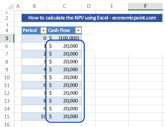
Here comes the tricky part, in Excel, the cash flow doesn’t include the initial investment. For example, if our cash flow is as follows:

We must not include “-100,000” (cell C5) in the actual Excel NPV formula, but only all the following values, and then subtract 100,000 from the result.

The Discount Rate in the NPV Formula

To use the NPV formula, we need a discount rate. A discount rate is usually the rate of return of the best alternative investment with a similar risk profile. For example, if we have an alternative investment with a rate of return of 5% yearly and the same risk as the investment we are currently analyzing, we should use 5% as the discount rate in the NPV formula.

So, there are two key data that we must know to use the NPV formula in Excel:
1- The Cash Flow (don’t forget to not include the initial investment in the actual NPV formula)
2- The Discount Date

Many Excel users do the mistake of including the initial investment in the actual NPV formula, and the difference with the right way to do it is minor. Because the difference is small, a lot of people get the wrong value and do not notice it.

Instructions to use the NPV formula in Excel

Knowing all this, let’s do it:

Step 1: Insert your Cash Flow

Insert all the cash flows. They can be calculated annually, monthly or using another time period, but you must take into account that the discount rate must correspond to the time period used in the cash flow.

For example, if you have years in your cash flow, you must use a discount rate expressed in years. To get a monthly rate from a yearly rate, use the following formula:

=(1+A1)^(1/12)-1

Where A1 is the cell that contains the yearly rate. For example, if you have a yearly rate of 20%, the monthly rate is near 1.53%. Note: in this example, the values are expressed in actual numbers: 0.20 is the yearly rate and 0.015309 the monthly rate.

Regarding the initial investment or the cash flow in period zero, I usually put this value in the same cash flow, but you can also use a cell distant from the future cash flow.

Step 2: Insert the Discount Rate

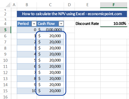
Afther entering the cash flow and the discount rate, your sheet will look like this one:

Step 3: Enter the NPV Excel Formula

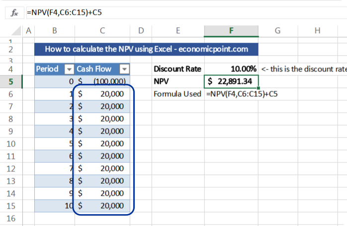
Insert “=NPV(E3,B5:B14)+B4”
where:
E3 is the cell containing the discount rate
B5:B14 is the range containing the future cash flows
B4: is the cell containing the initial investment

Working Example